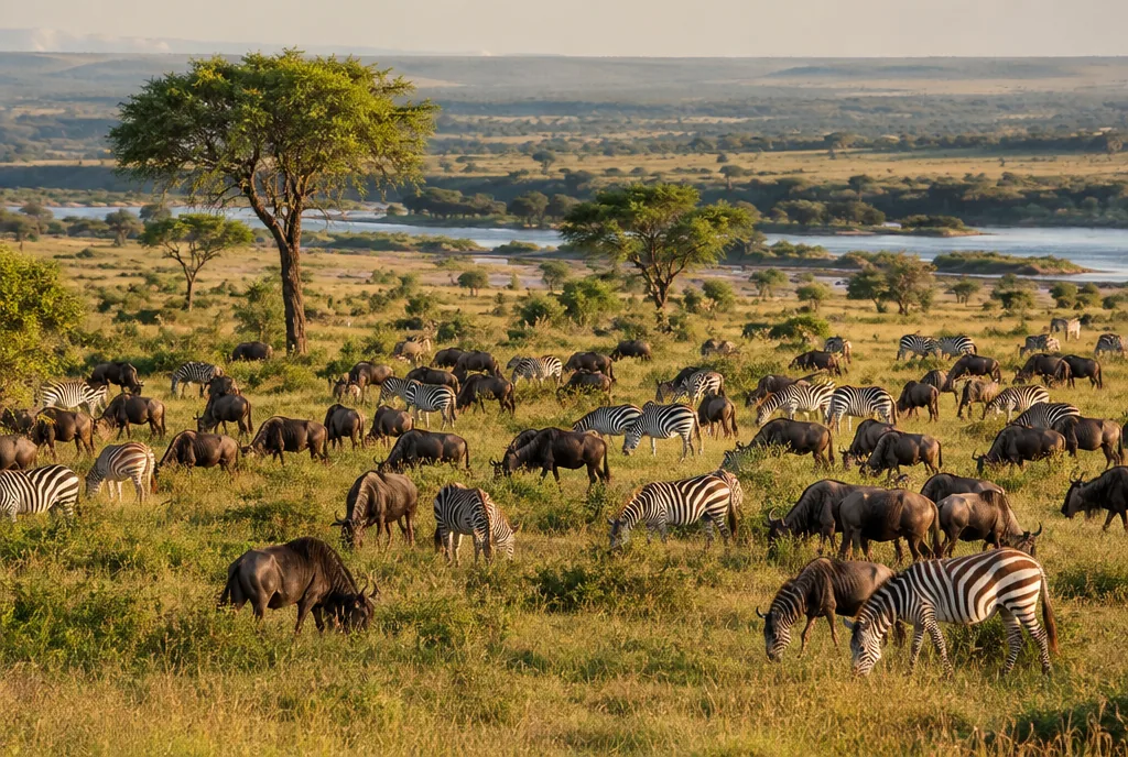
Population ecology is the branch of ecology that explains how a population changes in size, density, and structure across time and space. Its central question is deceptively simple: why are there more, fewer, or differently distributed members of one species in one place than before? The answer can connect a caterpillar’s host plant, a drought, a predator’s delayed response, and the age makeup of a population. By following those connections, population ecology turns a head count into a story about limits, opportunities, and change.
Start with the population, then ask what is changing
A population is examined through several characteristics at once. Population density is the number of individuals per unit of land area. Dispersion describes their spatial arrangement. Age structure shows how individuals are distributed among ages, while mating system and genetic variation describe features within the population’s gene pool. None of these measures alone explains a population, but together they establish what needs explanation.
Distribution adds another layer. A species’ geographic range is often not one continuous occupied space. It can be a patchwork of occupied and unoccupied areas because barriers restrict dispersal and microhabitats differ. Within that patchwork, local density can fluctuate as conditions change. The chinch bug in Illinois, for example, has shown density swings tied to habitat quality.
Population ecologists use mathematical models to describe such behavior. Exponential and logistic equations focus on growth, while Lotka-Volterra equations describe predator-prey relationships. Models do not replace observation. They provide a disciplined way to ask which conditions would produce the pattern seen in the field.
Population density and dispersion reveal where individuals can meet
Density matters because it gives a population’s abundance a spatial scale. A high count across a large region and the same count in a small area do not describe the same ecological situation. Human density makes the point vividly: averaged across land only, the worldwide figure is about 53 people per square kilometer, yet 95% of the world’s population is concentrated on 10% of its land area. Monaco, with 18,589 people per square kilometer on 2.02 square kilometers of land, sits at the other end of the contrast.
Dispersion asks how individuals are arranged inside the area they occupy. Ecologists recognize three recurring patterns.
| Pattern | What it looks like | What can produce it | Example |
|---|---|---|---|
| Clumped | Individuals occur in groups | Resources occur in patches or organisms form social groups | Pipevine swallowtail caterpillars gather where California pipevine, their host plant, grows. |
| Uniform | Individuals are spaced relatively evenly | Territoriality or competition | Desert cacti can be evenly spaced when intense competition for water keeps individuals apart. |
| Random | No clear spatial pattern | Resources are evenly distributed | This pattern is rare in nature. |
Repeated quadrat counts make those patterns measurable. Ecologists compare the sample mean and variance of organism counts from quadrats. This statistical comparison helps distinguish a clustered population from an evenly spaced or random one, rather than relying on an impression from a single walk through a habitat.
Exponential growth shows what r means under ideal conditions
In population ecology, r is the intrinsic rate of natural increase: the maximum per-capita growth rate under ideal, unconstrained conditions. It is also called the Malthusian parameter and can be calculated as births minus deaths per generation time. The letter comes from “rate,” while K comes from the German Kapazitätsgrenze, or capacity limit. This is not the same as finite rate of increase, R, which is the factor by which a population multiplies per time unit. A Paramecium population dividing twice each day has R = 2.
Exponential growth assumes a constant per-capita rate and unlimited resources. Its equation is Nt = N0 × e(rt), and its graph is J-shaped. The assumption is intentionally stark. A single pair of bacteria dividing every 20 minutes would create more than 5 × 10²⁰ individuals in 24 hours if that growth continued unchecked. The example makes the key lesson visible: a constant proportional increase becomes enormous quickly.
Thomas Malthus framed an early version of this problem by arguing that population grows exponentially while resources grow only linearly, creating a “struggle for existence.” Charles Darwin was profoundly influenced by Malthus in developing natural selection for On the Origin of Species. Population ecology retains the useful tension in that idea: growth potential is one part of the story; conditions that constrain it are the other.
Carrying capacity explains why growth often bends
Carrying capacity, represented by K, is the maximum population size that an environment can sustain indefinitely, at the equilibrium where births equal deaths. In the logistic equation, dN/dt = rN(1 − N/K), r governs exponential growth when a population is far below K. As N approaches K, the per-capita growth rate declines linearly, producing an S-shaped curve rather than a J-shaped one.
The logistic equation was first proposed by Belgian mathematician Pierre-François Verhulst in 1838. It also captures a useful consequence of overshooting the model’s limit: when N is greater than K, the term (1 − N/K) is negative, so the model predicts decline back toward K. A textbook example makes the parameter concrete. If 100 caterpillars can each host at most 80 parasitic wasps, the carrying capacity for the wasp population is 8,000.
Still, carrying capacity is not a universal, permanently fixed number waiting to be discovered. Ecologists have questioned its usefulness for wild populations because it can oversimplify complicated species interactions and assume resources are homogeneous. The term itself began in range management, where it described the density of stock that could graze without damaging the range. That origin is a reminder to ask: sustained by which environment, with which resources, and under which interactions?
Density-dependent and density-independent forces act differently
Some forces grow stronger as density increases; others do not. Density-dependent factors are biotic forces such as predation, competition, and disease. Their intensity rises with population density. A crowded population may therefore face stronger competition or faster disease transmission than a sparse one.
The reverse situation can also be dangerous. Positive density-dependence, called the Allee effect, occurs when per-capita growth declines at low density. Below a critical threshold, a small population can be pushed toward extinction. So fewer individuals do not always mean more room to recover.
Density-independent factors are typically abiotic events: weather, natural disasters, and insecticides. They affect a population regardless of how dense it is. Catastrophic mortality from weather, for instance, kills a constant proportion of individuals irrespective of population size. The distinction helps separate a response to crowding from a response to an external shock.
Life histories and survivorship show different routes through risk
The familiar labels r-selected and K-selected summarize contrasting life-history tendencies. r-selected species, including weeds, insects, and rodents, tend to have high reproductive rates, rapid development, and small body size. They thrive in unstable or unpredictable environments. K-selected species, including elephants, whales, and humans, tend to have low reproductive rates, slow development, and large body size, and they thrive in stable environments near carrying capacity.
MacArthur and Wilson formalized r/K selection theory in their theory of island biogeography. The labels remain useful shorthand, but they are not rigid bins. A review by Parry found no consensus on the exact definition of r- and K-selection, challenging the theory’s consistency. Used carefully, the terms describe a pattern; neither label is a complete identity for a species.
Survivorship curves supply another view of life history. Built from life tables for a cohort, they typically plot 1,000 starting individuals on a logarithmic y-axis against age on the x-axis.
- Type I: Most individuals survive to old age. Humans and elephants are typical examples.
- Type II: Mortality is constant at any age. Some birds and lizards show this pattern.
- Type III: Early mortality is very high, while survivors live long. Oysters produce millions of eggs, but most larvae die.
Predator-prey cycles make timing part of the explanation
Alfred Lotka and Vito Volterra independently developed the Lotka-Volterra predator-prey equations. These paired, first-order nonlinear differential equations put interaction at the center of population change. One historical observation that helped inspire Volterra was a report from marine biologist Umberto D’Ancona: shark and predatory fish populations increased during World War I when fishing was reduced.
The Hudson Bay Company record of Canadian lynx and snowshoe hare pelts from 1845 to 1935 offers a classic field-scale pattern. Across those 90 years, the populations showed cycles lasting roughly 8 to 11 years. Hare peaks came one to two years before lynx peaks. The delay matters: a predator population does not peak at the same instant as its prey.
Later work extended the basic framework. C. S. Holling developed the “disc curve” functional response to describe the rate at which predators consume prey as prey density changes. The Rosenzweig-MacArthur model added density-dependent prey growth and a Holling-type functional response. Each addition points to the same caution: a clean cycle is an entry point for investigation, not the whole ecological system.
Population ecology connects field counts to conservation and human growth
Population ecologists study population size, density, age structure, and interactions among species to identify what drives changes in abundance. Their work combines field research, data analysis, and mathematical modeling. Leslie matrix models, for example, are used for age-structured populations to project population trajectories and inform conservation. In pest management, an understanding of a pest’s r/K status can help integrate control strategies; most crop pests are r-strategists adapted to exploit unstable agroecosystems.
Human population growth also belongs in this frame, but it is not reducible to a single global K. The world population reached 8 billion in 2022, after taking 12 years to grow from 7 billion. United Nations projections indicated roughly 15 years to reach 9 billion, around 2037, followed by further slowing. About 70% of the population added between 7 and 8 billion was in low-income and lower-middle-income countries.
Resource use changes the question from head count alone to the relationship between population and biocapacity. The Global Footprint Network calculates that humanity has been in ecological overshoot since about 1970 and uses resources at about 170% of Earth’s annual regenerative capacity. The Planetary Boundaries framework identifies nine Earth-system processes; crossing their thresholds could permanently reduce Earth’s human carrying capacity. Those statements make carrying capacity a question about environment and consumption, not a numerical verdict on people.
Common misunderstandings obscure how populations actually change
“Carrying capacity is a fixed ceiling.”
In the logistic model, K is a parameter. In wild populations, complex interactions and uneven resources can make one fixed K an oversimplification. A population can also exceed K in the model and then decline.
“Every population grows exponentially.”
Exponential growth describes constant per-capita growth with unlimited resources. Logistic growth instead describes a declining per-capita rate as N approaches K. Predator-prey interactions and external shocks add still more possibilities.
“r-selected and K-selected are permanent species categories.”
They describe contrasting tendencies in life history, and their precise definitions have been disputed. Using them as a shortcut should never erase the environment or the traits being discussed.
Frequently Asked Questions
What is population ecology?
Population ecology is the study of how species populations change in size, density, and structure over time and space. It uses observations and models to examine growth, distribution, and interactions.
What are the characteristics of a population?
Key characteristics include density, dispersion, age structure, mating system, and genetic variation within the gene pool. Geographic distribution is often a patchwork shaped by dispersal barriers and microhabitat differences.
What is carrying capacity?
Carrying capacity, K, is the maximum population size an environment can sustain indefinitely, where births equal deaths. It is useful in the logistic model, but can oversimplify wild populations with changing resources and interactions.
What do population ecologists do?
They investigate population size, density, age structure, and interactions among species. Field research, data analysis, and models such as Leslie matrices help them project trajectories and inform conservation.
What is r in population ecology?
r is the intrinsic rate of natural increase: the maximum per-capita population growth rate under ideal, unconstrained conditions. In the logistic equation, it controls exponential growth when a population is far below carrying capacity.